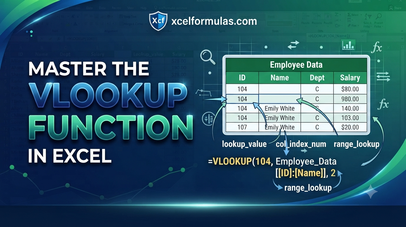
With VLOOKUP in Excel, you can quickly find a number in the first column of a table and get information from another related column. It makes it easier to work with big numbers, speeds up data lookup, and connects data across sheets.
What is VLOOKUP?
“VLOOKUP” stands for “vertical lookup.” It lets you find cells by looking at other cells. You can tell Excel or Google Sheets, “Find Abkhazia in this column [of the size sheet] and give me its area from the column next to it.” Oh, I see, Abkhazia is a disputed area on the eastern coast of the Black Sea. Interesting, huh?

It’s quite useful when your two sheets represent different countries, and you’re unable to simply copy the size column and paste it alongside the population column.
ALSO READ:
How does VLOOKUP work?
The VLOOKUP formula can be tricky, so let’s walk through it step by step.

Start by creating a column for the lookup results you want Excel to return. Since we want to display country sizes next to the population data, I will add a new column labeled “size” right beside it.
Next, type =VLOOKUP(). This tells Excel or Google Sheets that you intend to use this formula. It requires four parameters:
- Search key: What you are looking for (e.g., “Find Abkhazia…”).
- Range: Where to look (e.g., “…in this column…”).
- Index: Which value to return (e.g., “…return the size from the adjacent column.”).
- Is sorted: Whether your data is sorted alphabetically.
That may seem like a lot, but stay with me—we will go through it together.
VLOOKUP Formula Explained (Syntax of VLOOKUP)
The VLOOKUP formula follows this basic structure:
=VLOOKUP(lookup_value, table_array, col_index_num, [range_lookup])
Excel’s VLOOKUP function requires four arguments:
- Lookup_value: The value you want Excel to find in the lookup table.
- Table_array: The range or table where Excel should perform the search.
- Col_index_num: The specific column number that contains the data you want to retrieve.
- Range_lookup: A toggle to specify whether you want an exact or approximate match.
Mastering this formula helps avoid common issues, such as inaccurate results or missing data. Most users prefer an exact match by setting the final argument to FALSE, which ensures greater precision.
Step-by-Step Guide: How to Use VLOOKUP in Excel
Step 1: Use the Provided Excel Data
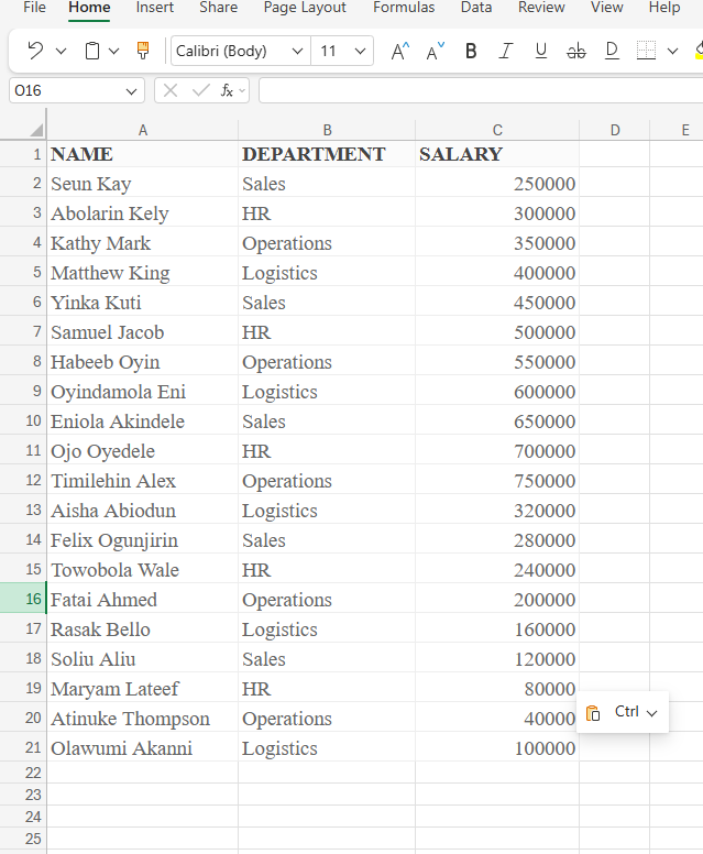
Step 2: Determine Your Search Criteria
In this tutorial, we will:
- Search for a specific employee’s name.
- Retrieve their corresponding salary or department.
Example: Find the salary for “Kathy Mark.”
Step 3: Set Up a Lookup Area
Navigate to an empty section of your spreadsheet (e.g., columns E and F).
Enter the following headers:
- E2: Employee Name
- F2: Salary
In cell E3, type the name you wish to look up (e.g., “Kathy Mark”).
Step 4: Enter the VLOOKUP Formula
Click on cell F3 (where you want the result to appear) and enter the following formula:
=VLOOKUP(E3, A2:C21, 3, FALSE)
Formula Breakdown:
- E3: The value you are searching for.
- A2:C21: The data table range.
- 3: The column index containing the salary.
- FALSE: Specifies an exact match.
Press Enter, and Excel will display 350,000, the salary associated with Kathy Mark.

Step 5: Look Up the Department Instead
To retrieve the department instead of the salary, use the following formula:
Press F3 and change the formula to:
=VLOOKUP(E3, A2:C21, 2, FALSE)
Reasoning:
Column 2 contains the DEPARTMENT.
Excel will now return: Operations

Step 6: Practice with Other Names
Replace the name in cell E3 with:
- Seun Kay
- Yinka Kuti
- Maryam Lateef
The formula will automatically display the matching department or salary for the selected employee.
Important VLOOKUP Tips
- Make sure the NAME column is the first column in the table you select. VLOOKUP uses this column to find the information you need.
- VLOOKUP cannot search from right to left.
- Always use FALSE unless you specifically require an approximate match.
- Names must be spelled identically for an exact match to work correctly.
Common VLOOKUP Errors in Excel
#N/A: This usually means Excel couldn’t find the name in your list. Check the spelling and spaces to make sure they match exactly.
Conclusion
Using VLOOKUP with employee data makes it easy to find salaries, departments, and other details quickly. Once you understand how the formula works and how to use column numbers, VLOOKUP can become a helpful tool for managing data in Excel.